Python을 이용한 국내 전기차 충전소 수요 예측 분석 및 시각화
from google.colab import files
uploaded = files.upload()
# Saving 연도별 친환경자동차 등록현황.csv to 연도별 친환경자동차 등록현황.csv

from google.colab import files
uploaded = files.upload()
# Saving 연료종류별 자동차 등록현황.csv to 연료종류별 자동차 등록현황.csv

from google.colab import files
uploaded = files.upload()
# Saving 지역별 주유소 현황.csv to 지역별 주유소 현황.csv
import pandas as pd
import numpy as np
import matplotlib.pyplot as plt
import seaborn as sns
import matplotlib.patches as patches
import plotly.graph_objects as go
from datetime import datetime
from plotnine import *
from pandas.tseries.offsets import YearEnd
from sklearn.linear_model import LinearRegression# 한글 폰트 깨짐 현상 해결 (실행 후 > 런타임 > 런타임 다시 시작)
!sudo apt-get install -y fonts-nanum
!sudo fc-cache -fv
!rm ~/.cache/matplotlib -rf
plt.rc('font', family = 'NanumBarunGothic')############ 옵션 parameter ############
# 예측할 년도 범위
start_year = 2025 # start_year ~ end_year의 데이터 예측 (이상, 이하)
end_year = 2050 # start_year ~ end_year의 데이터 예측 (이상, 이하)
gap_year = 5 # 연 간격
# 주유소 수용률 계산용
gas_gun = 8 # 주유소당 평균 주유기 개수
elec_time = 200 # 한 대의 전기차가 충전을 위해 머무는 시간 (분)
gas_time = 5 # 한 대의 전기차가 충전을 위해 머무는 시간 (분)
#######################################
Ⅰ. CSV 읽기
eco_df = pd.read_csv('연도별 친환경자동차 등록현황.csv', encoding = 'cp949', index_col = 0, header = None, thousands = ',').T
car_df = pd.read_csv('연료종류별 자동차 등록현황.csv', encoding = 'cp949', index_col = 0, header = None, thousands = ',').T
gas_station_df = pd.read_csv('지역별 주유소 현황.csv', encoding = 'cp949', index_col = 0, header = None, thousands = ',').T

year_range = range(start_year, end_year+1, gap_year)
X_predict = pd.DataFrame(data = [datetime.toordinal(datetime(_,12,31)) for _ in year_range], columns = ['연도'])
Ⅱ. 데이터 시각화
eco_df.head(8)| 연도 | 친환경계 | 하이브리드차 | 전기차 | 수소차 | |
| 1 | 2013 | 105044 | 103580 | 1464 | 0 |
| 2 | 2014 | 140297 | 137522 | 2775 | 0 |
| 3 | 2015 | 180361 | 174620 | 5712 | 29 |
| 4 | 2016 | 244158 | 233216 | 10855 | 87 |
| 5 | 2017 | 339134 | 313856 | 25108 | 170 |
| 6 | 2018 | 461733 | 405084 | 55756 | 893 |
| 7 | 2019 | 601048 | 506047 | 89918 | 5083 |
| 8 | 2020 | 820329 | 674461 | 134962 | 10906 |
fig = plt.figure()
plt.figure(figsize = (10, 7)) # 그래프 크기
plt.rc('font', size = 15) # 폰트 크기
titleFont = {'fontsize': 20, 'color': '#000000'} # 제목 폰트 설정

# x축 연도 : y축 친환경자동차 등록현황
plt.plot(eco_df['연도'], eco_df['친환경계'], color = 'black', marker = 'o', label = '친환경계', linestyle = 'solid')
plt.plot(eco_df['연도'], eco_df['하이브리드차'], color = 'blue', marker = '.', label = '하이브리드차' , linestyle = 'solid')
plt.plot(eco_df['연도'], eco_df['전기차'], color = 'red', marker = 'x', label = '전기차',linestyle = 'solid')
plt.plot(eco_df['연도'], eco_df['수소차'], color = 'green', marker = '.', label = '수소차', linestyle = 'solid')

# 제목
plt.title("연간 친환경자동차 등록현황", fontdict = titleFont)

# 범례, 그리드
plt.legend(loc='upper left')
plt.grid(True)

# x축 y축 레이블
plt.xlabel("연도")
plt.ylabel("자동차 등록수")

# 전기차 데이터 표시
for i in range(1, 9):
  plt.annotate(eco_df['전기차'][i], (2012 + i, eco_df['전기차'][i]), textcoords = "offset points", xytext = (0, 5), ha = 'center')

plt.show()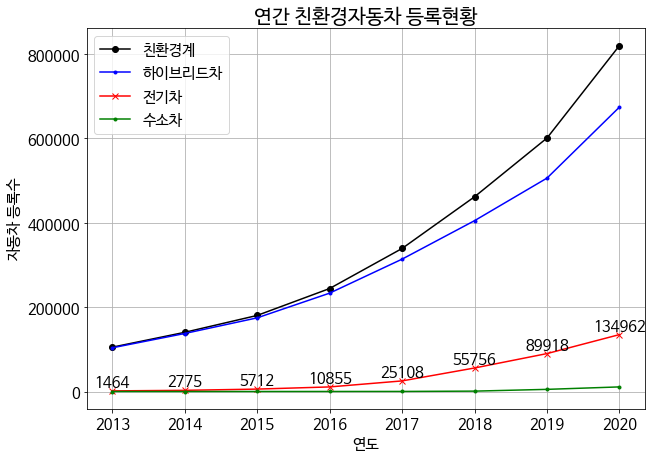
car_df.head(7)| 연도 | 차량계 | 휘발유 | 경유 | LPG | 하이브리드 | CNG | 전기 | |
| 1 | 2014 | 20117955 | 9587351 | 7938627 | 2336656 | 137522 | 40457 | 2775 |
| 2 | 2015 | 20989885 | 9808633 | 8622179 | 2257447 | 174620 | 39777 | 5712 |
| 3 | 2016 | 21803351 | 10092399 | 9170456 | 2167094 | 233216 | 38880 | 10855 |
| 4 | 2017 | 22528295 | 10369752 | 9576395 | 2104675 | 313856 | 38918 | 25108 |
| 5 | 2018 | 23202555 | 10629296 | 9929537 | 2035403 | 405084 | 38934 | 55756 |
| 6 | 2019 | 23677366 | 10960779 | 9957543 | 2004730 | 506047 | 38147 | 89918 |
| 7 | 2020 | 24365979 | 11410484 | 9992124 | 1979407 | 674461 | 36940 | 134962 |
fig = plt.figure()
plt.figure(figsize = (20, 7)) # 그래프 크기
plt.rc('font', size = 15) # 폰트 크기

### 연도별 누적 합계 그래프 ###
x1 = car_df['휘발유']
x2 = car_df['경유']
x3 = car_df['LPG']
x4 = car_df['하이브리드']
x5 = car_df['CNG']
x6 = car_df['전기']
x7 = car_df['수소']
x8 = car_df['기타']

data = [x1, x2, x3, x4, x5, x6, x7, x8]
x_array = car_df['연도']

plt.subplot(1, 2, 1)  # 누적 합계 그래프 배치
for i in range(0, 8): # 누적 막대 데이터 8개
  plt.bar(
    x_array,          # 0부터 8까지의 X 위치에서
    data[i],          # 각 높이(8개)만큼 쌓음
    bottom = np.sum(data[:i], axis=0)
  )

# 제목
plt.title("연간 연료종류별 자동차 등록현황", fontdict = titleFont)

# x축 y축 레이블
plt.xlabel("연도")
plt.ylabel("연료종류별 자동차 등록수 (단위 : 천만)") #2.5 -> 2천 5백만
plt.ylim([0, 27500000]) #y축 공간 여백

# 화살표
arrow = patches.FancyArrowPatch(
    (2020, 28000000), # 화살표 X축
    (2020, 25000000), # 화살표 Y축
    mutation_scale = 20,
    color = 'red',
    fill = True,
    alpha = 100)
plt.gca().add_patch(arrow)


### 2020년 연료종류별 자동차 등록현황 원형 그래프 ###
names = ['휘발유 (11,410,484)', '경유 (9,992,124)', 'LPG (1,979,407)', '전기 (134,962)', '하이브리드 (67만), CNG (4만), 수소 (1만), 기타 (13만)']
values = [11410484, 9992124, 1979407, 134962, 674461 + 36940 + 10906 + 126695]

plt.subplot(1, 2, 2)  # 원형 그래프 배치

# 제목
plt.text(-1.05, 1.15, '[2020년 연료종류별 자동차 등록현황]', fontdict = titleFont)

# 레이블
plt.pie(values, labels=names, labeldistance = 1.05);

plt.show()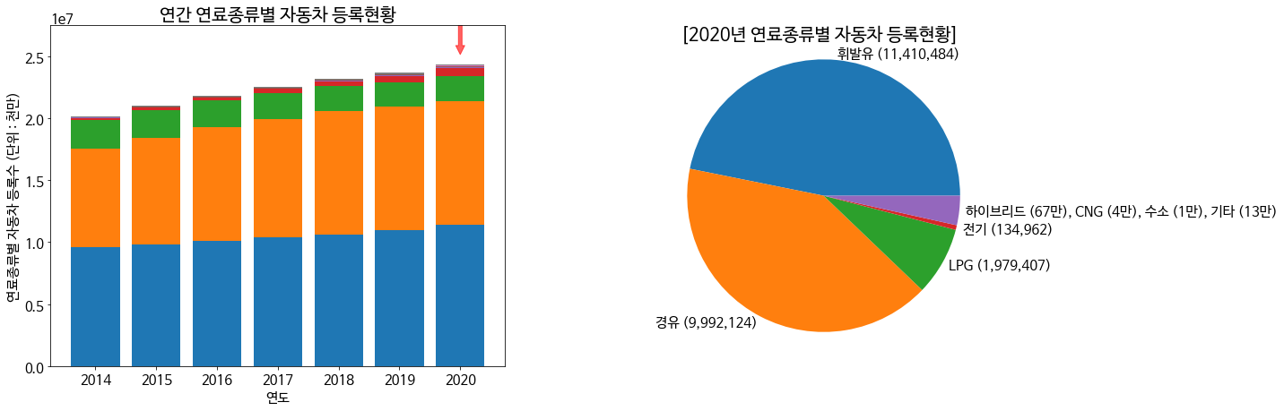
| 연도 | 강원도 | 경기도 | 경상남도 | 경상북도 | 광주광역시 | 대구광역시 | 대전광역시 | 부산광역시 | 서울특별시 | 세종특별자치시 | 울산광역시 | 인천광역시 | 전라남도 | 전라북도 | 제주도 | 충청남도 | 충청북도 | 주유소계 | |
| 1 | 2017 | 708 | 2426 | 1166 | 1314 | 288 | 374 | 251 | 433 | 537 | 64 | 250 | 349 | 926 | 918 | 193 | 1055 | 755 | 12007 |
| 2 | 2018 | 681 | 2386 | 1150 | 1278 | 280 | 369 | 240 | 427 | 508 | 64 | 244 | 346 | 904 | 906 | 193 | 1034 | 740 | 11750 |
| 3 | 2019 | 674 | 2396 | 1135 | 1287 | 277 | 364 | 240 | 416 | 496 | 66 | 239 | 342 | 902 | 903 | 194 | 1033 | 736 | 11700 |
| 4 | 2020 | 675 | 2391 | 1117 | 1263 | 269 | 348 | 236 | 403 | 488 | 68 | 240 | 336 | 899 | 902 | 194 | 1026 | 734 | 11589 |
| 5 | 2021 | 659 | 2361 | 1090 | 1264 | 262 | 343 | 227 | 387 | 470 | 69 | 237 | 330 | 877 | 883 | 194 | 1008 | 717 | 11378 |
| 6 | 2022 | 642 | 2330 | 1071 | 1246 | 260 | 332 | 220 | 380 | 442 | 67 | 234 | 323 | 869 | 856 | 194 | 1002 | 713 | 11181 |
fig = plt.figure()
plt.figure(figsize = (20, 10)) # 그래프 크기
plt.rc('font', size = 15) # 폰트 크기

# 2022년 데이터 입력
labels = ['강원도', '경기도', '경상남도', '경상북도', '광주광역시', '대구광역시', '대전광역시', '부산광역시	', '서울특별시', '세종특별자치시', '울산광역시', '인천광역시', '전라남도', '전라북도', '제주도', '충청남도', '충청북도']
sizes = [642, 2330, 1071, 1246, 260, 332, 220, 380, 442, 67, 234, 323, 869, 856, 194, 1002, 713]
explode = (0, 0.1, 0, 0, 0, 0, 0, 0, 0, 0, 0, 0, 0, 0, 0, 0, 0)

# 제목
plt.title("[2022년 지역별 주유소 비율]", fontdict = titleFont)

plt.pie(sizes,
        explode = explode,
        labels = labels,
        autopct = '%1.0f%%',
        shadow = True,
        labeldistance = 1.05,
        startangle = 90)

plt.axis('equal') # 비율 반영
plt.show()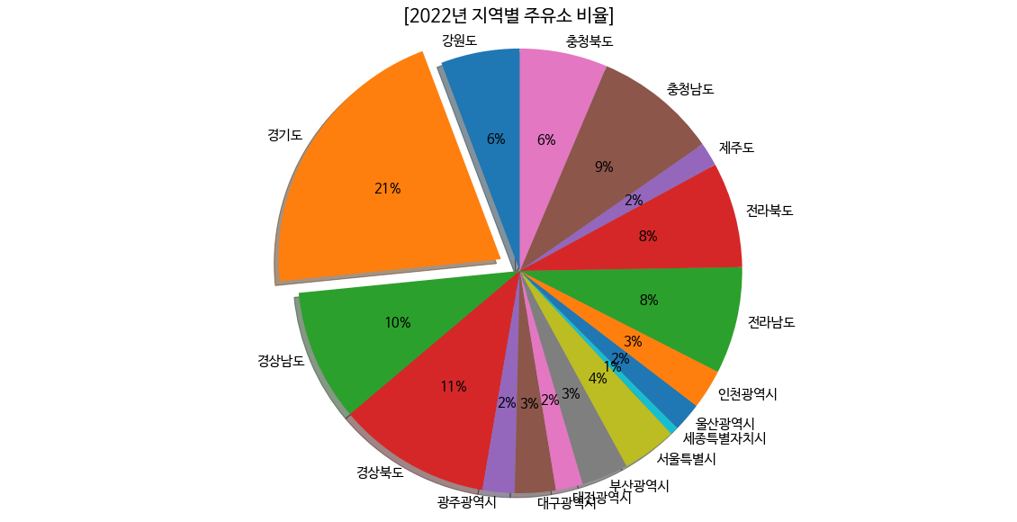
year_range
# range(2025, 2051, 5)X_predict| 연도 | |
| 0 | 739616 |
| 1 | 741442 |
| 2 | 743268 |
| 3 | 745095 |
| 4 | 746921 |
| 5 | 748747 |
Ⅲ. 총 차량 수 예측
# 연도를 학습에 맞게 ordinal로 변경(데이터 전처리)
car_df['연도'] = pd.to_datetime(car_df['연도'], format = '%Y') + YearEnd(0)
car_df['연도'] = car_df['연도'].apply(datetime.toordinal)

# 데이터셋
total_car_X = car_df[['연도']]
total_car_Y = car_df[['차량계']]

# 예측 모델
total_car_lr = LinearRegression()

# 예측 모델 학습
total_car_lr.fit(total_car_X, total_car_Y)

# 예측
total_car_Y_predict = total_car_lr.predict(X_predict).round()

# 0 미만은 0으로 변경
total_car_Y_predict[total_car_Y_predict < 0] = 0
Ⅳ. 총 전기차 수, 친환경차량 수 예측
# 연도를 학습에 맞게 ordinal로 변경
eco_df['연도'] = pd.to_datetime(eco_df['연도'], format = '%Y') + YearEnd(0)
eco_df['연도'] = eco_df['연도'].apply(datetime.toordinal)

# 데이터셋
eco_X = eco_df[['연도']]
elec_Y = eco_df[['전기차']]
eco_Y = eco_df[['친환경계']]

# 예측 모델
elec_lr = LinearRegression()
eco_lr = LinearRegression()

# 예측 모델 학습
elec_lr.fit(eco_X, elec_Y)
eco_lr.fit(eco_X, eco_Y)

# 예측
elec_Y_predict = elec_lr.predict(X_predict).round()
eco_Y_predict = elec_lr.predict(X_predict).round()

# 0 미만은 0으로 변경
elec_Y_predict[elec_Y_predict < 0] = 0
eco_Y_predict[eco_Y_predict < 0] = 0
Ⅴ. 총 주유소 수 예측
# 연도를 학습에 맞게 ordinal로 변경
gas_station_df['연도'] = pd.to_datetime(gas_station_df['연도'], format = '%Y') + YearEnd(0)
gas_station_df['연도'] = gas_station_df['연도'].apply(datetime.toordinal)

# 데이터셋
gas_station_X = gas_station_df[['연도']]
gas_station_Y = gas_station_df[['주유소계']]

# 예측 모델
gas_station_lr = LinearRegression()

# 예측 모델 학습
gas_station_lr.fit(gas_station_X, gas_station_Y)

# 예측
gas_station_Y_predict = gas_station_lr.predict(X_predict).round()

# 0 미만은 0으로 변경
gas_station_Y_predict[gas_station_Y_predict < 0] = 0
Ⅵ. 주유소 평균 수용률 계산
(전국 주유소 개수 / 전국 차량 대수)
ratio_df = pd.merge(car_df, gas_station_df[['연도','주유소계']], on = '연도')
gas_car_list = ['휘발유', '경유', 'LPG', '하이브리드', 'CNG']
ratio_df['화석차계'] = ratio_df[gas_car_list].sum(axis=1)
ratio_df['수용률'] = ratio_df['주유소계'] / ratio_df['화석차계'] * gas_gun * elec_time / gas_time

mean_acc = ratio_df["수용률"].mean()
[수용률 계산 데이터]
ratio_df['주유소계'] : 12007 11750 11700 11589
ratio_df['화석차계'] : 22403596 23038254 23467246 24093416
gas_gun : 8
elec_time : 200
gas_time : 5
= ratio_df['수용률'] : 0.171501 0.163207 0.159542 0.153921
Ⅶ. 예측 결과 출력
print(f'화석 차량 주유소 평균 수용률 : {mean_acc}')

y_predict_list = [
    ('총 차량 수', total_car_Y_predict.round()),
    ('친환경 자동차 수', eco_Y_predict.round()),
    ('전기 자동차 수', elec_Y_predict.round()),
    ('주유소 수', gas_station_Y_predict.round()),
    ('필요한 전기차 충전기 수', (eco_Y_predict * mean_acc).round())
]

for i, year in enumerate(year_range):
    print(f'\n- {year}년')
    for item in y_predict_list:
        print(f'{item[0]} : {int(item[1][i]):,}')
화석 차량 주유소 평균 수용률 : 0.16204256407658063
- 2025년
총 차량 수 : 27,960,043
친환경 자동차 수 : 196,109
전기 자동차 수 : 196,109
주유소 수 : 10,759
필요한 전기차 충전기 수 : 31,778
- 2030년
총 차량 수 : 31,444,657
친환경 자동차 수 : 287,439
전기 자동차 수 : 287,439
주유소 수 : 9,994
필요한 전기차 충전기 수 : 46,577
- 2035년
총 차량 수 : 34,929,270
친환경 자동차 수 : 378,770
전기 자동차 수 : 378,770
주유소 수 : 9,229
필요한 전기차 충전기 수 : 61,377
- 2040년
총 차량 수 : 38,415,791
친환경 자동차 수 : 470,151
전기 자동차 수 : 470,151
주유소 수 : 8,463
필요한 전기차 충전기 수 : 76,184
- 2045년
총 차량 수 : 41,900,404
친환경 자동차 수 : 561,482
전기 자동차 수 : 561,482
주유소 수 : 7,698
필요한 전기차 충전기 수 : 90,984
- 2050년
총 차량 수 : 45,385,017
친환경 자동차 수 : 652,812
전기 자동차 수 : 652,812
주유소 수 : 6,933
필요한 전기차 충전기 수 : 105,783
Ⅷ. 예측 결과 시각화
y_predict_df = pd.DataFrame({
    '연도': ['2025', '2030', '2035', '2040', '2045', '2050'],
    '총 차량 수': ['27,960,043', '31,444,657', '34,929,270', '38,415,791', '41,900,404', '45,385,017'],
    '친환경 자동차 수': ['196,109', '287,439', '378,770', '470,151', '561,482', '652,812'],
    '전기 자동차 수': ['196,109', '287,439', '378,770', '470,151', '561,482', '652,812'],
    '주유소 수': ['10,759', '9,994', '9,229', '8,463', '7,698', '6,933'],
    '필요한 전기차 충전기 수': ['31,778', '46,577', '61,377', '76,184', '90,984', '105,783'],
})
fig = plt.figure()
plt.rcParams['figure.figsize'] = (20, 7) # 그래프 크기
plt.rcParams['font.size'] = 15 # 폰트 크기
# 스타일 설정
plt.style.use('default')
# 데이터 준비
x = y_predict_df['연도']
y1 = y_predict_df['전기 자동차 수']
y2 = y_predict_df['필요한 전기차 충전기 수']
# 그래프 그리기
fig, ax1 = plt.subplots()
# 제목
plt.title("전기차 수와 필요한 전기차 충전기 수 예측", fontsize = 15, family = 'NanumBarunGothic')
# 필요한 전기차 충전기 수 그래프
ax1.plot(x, y1, color = 'red', alpha=0.7)
ax1.set_xlabel('연도', family = 'NanumBarunGothic')
ax1.set_ylabel('필요한 전기차 충전기 수', family = 'NanumBarunGothic')
ax1.tick_params(axis = 'both', direction='in')
# 전기 자동차 수 그래프
ax2 = ax1.twinx()
ax2.bar(x, y2, width = 0.7)
ax2.set_ylabel('전기 자동차 수', family = 'NanumBarunGothic')
ax2.tick_params(axis = 'y', direction = 'in')
ax2.set_ylim(0, 20)
plt.show()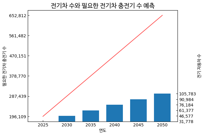
fig = plt.figure()
plt.figure(figsize = (10, 7)) # 그래프 크기
plt.rc('font', size = 10) # 폰트 크기

plt.subplot(2, 2, 1)
plt.plot(y_predict_df['연도'], y_predict_df['총 차량 수'], color = 'black', marker = 'o', label = '총 차량', linestyle = 'solid')
plt.legend(loc='upper left')
plt.grid(True)

plt.subplot(2, 2, 2)
plt.ylim(5.25, -0.25)
plt.plot(y_predict_df['연도'], y_predict_df['주유소 수'], color = 'black', marker = '.', label = '주유소', linestyle = 'solid')
plt.legend(loc='upper right')
plt.grid(True)

plt.subplot(2, 2, 3)
plt.plot(y_predict_df['연도'], y_predict_df['전기 자동차 수'], color = 'red', marker = 'x', label = '전기 자동차', linestyle = 'solid')
plt.legend(loc='upper left')
plt.grid(True)

plt.subplot(2, 2, 4)
plt.plot(y_predict_df['연도'], y_predict_df['필요한 전기차 충전기 수'], color = 'blue', marker = '.', label = '필요한 전기차 충전기', linestyle = 'solid')
plt.legend(loc='upper left')
plt.grid(True)

# 제목
plt.text(-5, 12.3, '[연간 총 차량, 주유소, 전기차, 충전기 변화율]', fontdict = titleFont)

plt.show()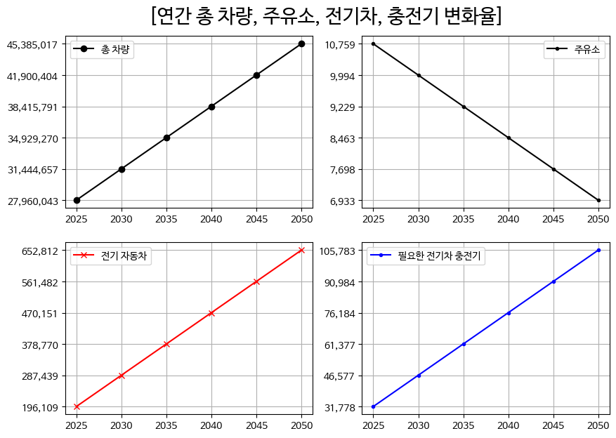
Ⅸ. 예측 결과 데이터 내보내기
y_predict_df.to_csv('2025년 2050년 5년 단위 예측 결과.csv',encoding="cp949", index = False) # 경로를 지정해서 파일 저장
!ls # 저장 확인
from google.colab import files
uploaded = files.upload()import io
predict_df = pd.read_csv(io.StringIO(uploaded['2025년 2050년 5년 단위 예측 결과 행렬전환.csv'].decode('cp949')), index_col = 0, header = None, thousands = ',').T