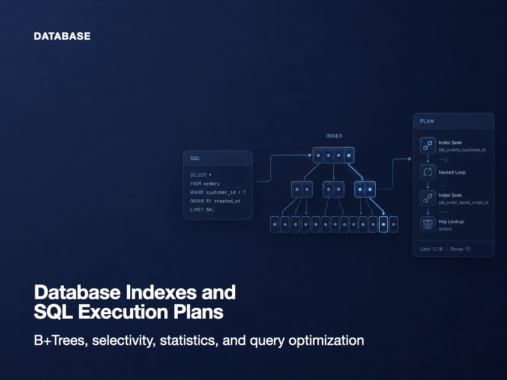
Database Indexes and SQL Execution Plans
Suppose we have the following orders table:
CREATE TABLE orders (
    order_id BIGINT PRIMARY KEY,
    customer_id BIGINT NOT NULL,
    order_status VARCHAR(20) NOT NULL,
    ordered_at DATETIME NOT NULL,
    total_amount BIGINT NOT NULL
);
When the table contains only a few hundred rows, the following query returns almost immediately:
SELECT *
FROM orders
WHERE customer_id = 1001;
The situation changes when the table grows to ten million rows.
Without an index on customer_id, the database may need to inspect a large portion of the table to find the matching orders.
Check order 1
Check order 2
Check order 3
...
Check order 10,000,000
With an appropriate index, the database may locate the relevant range without reading the table from beginning to end.
CREATE INDEX idx_orders_customer
ON orders (customer_id);
Does that mean every query becomes faster as soon as an index exists?
No.
A database may choose not to use an index when:
- the condition matches most of the table
- a function is applied to the indexed column
- the query skips the leading column of a composite index
- implicit type conversion interferes with index access
- statistics do not reflect the current data distribution
- a full table scan is estimated to be cheaper
- fetching many rows through the index causes excessive table lookups
- another access path better supports sorting, grouping, or joining
An index is not a command that forces the database to use a particular path.
When a database receives SQL, it considers multiple ways to execute the query and chooses the plan with the lowest estimated cost. The component responsible for this decision is the query optimizer.
To understand SQL performance, we therefore need to answer two related questions:
How does an index organize data for efficient access?
How does the optimizer choose among the available access paths?
An index creates possible paths.
An execution plan shows which path the database selected.
An index is a separate search structure
Imagine trying to find a particular term in a large book.
Without an index, we may have to inspect every page.
Check page 1
Check page 2
Check page 3
...
Check the final page
With an index at the back of the book, we can find the term and jump directly to the relevant page.
Transaction → page 142
Index → page 218
Normalization → page 95
A database index plays a similar role.
It is a separate search structure maintained alongside the table. Conceptually, it stores:
Index key
→ information used to locate the corresponding row
An index on customer_id might be represented like this:
1001 → row location
1001 → row location
1002 → row location
1003 → row location
The database searches the ordered index for 1001, identifies the matching range, and then retrieves the corresponding rows.
Without an index:
Read the table
→ inspect customer_id in each row
→ keep rows where customer_id = 1001
With an index:
Search the customer_id index for 1001
→ locate the matching index range
→ retrieve the required orders
The index does not replace the original table.
It creates an additional path to the data.
The purpose of an index is to reduce the search space
Suppose the table contains ten million orders, but Isaac has only twenty of them.
Without an index, the database might inspect ten million rows to return twenty.
Rows inspected: 10,000,000
Rows returned: 20
With a useful index, the database can locate the relevant key range and access only the required rows.
Search the index
→ locate Isaac's customer ID
→ retrieve twenty orders
The performance difference is not limited to the number of comparisons.
Database query cost may include:
- storage-page reads
- buffer-pool access
- index-page traversal
- row lookups
- CPU filtering
- sorting
- temporary-table creation
- network transfer
- locking and concurrency-control overhead
Indexes are especially valuable because they can reduce the number of pages that must be read.
Databases read pages, not isolated rows
SQL makes it appear as though the database reads one row at a time.
Storage engines, however, generally manage data in units called pages or blocks.
Data page
├── Row 1
├── Row 2
├── Row 3
└── Row 4
When the database reads the page containing one required row, other rows on the same page are loaded as well.
For this reason, three numbers may be very different:
Rows returned
≠
Rows examined
≠
Pages read
An efficient index helps the engine reach the right pages while avoiding unnecessary reads.
B-Trees and B+Trees provide balanced search
Relational databases commonly use B-Tree-family structures for general-purpose indexes.
Many storage engines use a structure based on the B+Tree.
A simplified tree might look like this:
                 [30 | 60]
                /    |    \
        [10 | 20] [40 | 50] [70 | 80 | 90]
Upper nodes contain separator keys that guide traversal.
Leaf nodes contain actual index keys and information used to locate the corresponding rows.
Root node
→ internal node
→ leaf node
→ row or row identifier
A balanced tree keeps traversal depth under control
A B+Tree maintains roughly the same distance from the root to every leaf.
It does not grow into a long one-sided chain.
100 rows
→ a small number of traversal steps

1,000,000 rows
→ far more data, but only a limited increase in tree height
This is why a large database can still locate a specific key using relatively few page accesses.
Each node stores many keys
A binary search tree typically has at most two children per node.
A B+Tree node can store many keys and child pointers in one page.
[100 | 200 | 300 | 400]
One page read therefore provides enough information to choose among many possible subtrees.
This high branching factor makes B+Trees suitable for storage systems where page access is expensive.
Leaf nodes are linked in key order
B+Tree leaf nodes can be linked sequentially.
[10, 20] ↔ [30, 40] ↔ [50, 60] ↔ [70, 80]
This is especially useful for range scans.
SELECT *
FROM orders
WHERE ordered_at >= '2026-07-01'
  AND ordered_at <  '2026-08-01';
The database can locate the first value in the range and then move through adjacent leaf entries until the upper boundary is reached.
This makes B+Tree indexes useful for:
- equality lookups
- range conditions
- ordered retrieval
- minimum and maximum searches
- prefix-based searches
B-Tree and B+Tree are related but different
Textbooks and certification exams may distinguish the two structures.
B-Tree
Both internal and leaf nodes may contain records or pointers to records.
A search may finish before reaching a leaf node.
B+Tree
Internal nodes are primarily used for navigation.
The data-access information is concentrated in the leaf nodes, and leaf nodes are linked in order.
B-Tree
A search may finish at an internal node

B+Tree
Data access is concentrated at leaf nodes
Linked leaves support efficient range scans
Implementation details differ among database products, but B+Tree concepts are central to understanding conventional relational indexes.
Hash indexes are strong at exact matching
A hash index applies a hash function to the key and uses the result to locate a bucket.
hash(customer_id)
→ bucket location
This can be efficient for exact equality conditions:
WHERE customer_id = 1001
A hash index does not naturally preserve key order.
It is therefore generally unsuitable for operations such as:
WHERE customer_id BETWEEN 1000 AND 2000;

ORDER BY customer_id;

WHERE customer_id > 1000;
A simple comparison is:
Strength
Exact equality lookup

Weakness
Range search
Sorting
Prefix search
Minimum and maximum lookup
Support for hash indexes varies by database and storage engine.
An index resembles an ordered copy of selected columns
Consider this table:
| order_id | customer_id | ordered_at |
| 1 | 1003 | 2026-07-03 |
| 2 | 1001 | 2026-07-01 |
| 3 | 1002 | 2026-07-02 |
| 4 | 1001 | 2026-07-04 |
An index on customer_id may conceptually store:
| customer_id | Row location or primary key |
| 1001 | 2 |
| 1001 | 4 |
| 1002 | 3 |
| 1003 | 1 |
The physical order of the table and the key order of the index may differ.
The database first finds matching index entries and then follows them to the table rows.
Read index
→ identify row locations
→ read base-table rows
That second step has a cost.
When a condition matches many rows, repeatedly jumping from the index to the table may be more expensive than scanning the table sequentially.
Clustered indexes are closely tied to row storage
A clustered index is closely associated with the physical organization of table rows.
Conceptually, the leaf level contains the actual row data.
Clustered-index leaf
→ complete table row
A table can normally have only one primary physical ordering.
In InnoDB-family storage engines, table data is organized around the primary key.
Primary-key index
→ row data stored at the leaf level
When a table has no explicit primary key, the engine may choose another suitable unique key or create an internal identifier.
Secondary indexes may locate rows through the primary key
In InnoDB-family engines, a secondary-index leaf entry contains the primary-key value.
For example:
Secondary index on customer_id

customer_id = 1001
→ order_id = 20035
→ search the primary-key index for order_id 20035
→ retrieve the complete order row
This can require two tree traversals:
1. Search the secondary index
2. Search the clustered primary-key index
If a query matches many rows and requests many columns, these repeated lookups can become expensive.
When every required column is already present in the secondary index, the database may avoid the second lookup.
That leads to the concept of a covering index.
Index access and full table scans
A database may consider several ways to access a table.
Full table scan
A full scan reads most or all table pages in sequence.
First orders page
→ next page
→ next page
→ final page
A full table scan is not automatically bad.
It may be the best choice when:
- the table is small
- most rows must be returned
- no useful index exists
- index lookups would require too many table accesses
- sequential I/O is cheaper than many random lookups
- an aggregate needs nearly the entire table
If a query must return nine million rows from a ten-million-row table, reading the table sequentially may be more efficient than performing nine million indexed row lookups.
Index lookup
The engine follows the index tree to a specific key or key range.
Root
→ internal node
→ leaf node
→ matching key range
This is often useful when the query returns a small portion of the table.
Full index scan
The database may scan the entire index rather than the table.
This can be beneficial when the index is much smaller than the table or when the index covers all required columns.
Range scan
A range scan locates a starting key and reads index entries until the end boundary.
SELECT order_id, ordered_at
FROM orders
WHERE ordered_at >= '2026-07-01'
  AND ordered_at <  '2026-08-01';
Locate 2026-07-01
→ read July entries in order
→ stop at 2026-08-01
Selectivity measures how strongly a condition reduces data
A key concept in index usefulness is selectivity.
It can be thought of as:
Selectivity
= matching rows / total rows
Suppose a query finds one order by a unique order ID:
1 / 10,000,000
Only a tiny fraction of the table is selected, so an index is highly useful.
Now suppose 90% of the orders have the status COMPLETED.
9,000,000 / 10,000,000
The following query does not reduce the table very much:
SELECT *
FROM orders
WHERE order_status = 'COMPLETED';
The optimizer may decide that a full scan is cheaper.
A useful generalization is:
Very few matching rows
→ index access is often attractive

Most rows match
→ a full scan may be more efficient
There is no universal percentage at which the decision changes.
The result depends on:
- row size
- index width
- cache state
- requested columns
- storage performance
- statistics
- access locality
Cardinality describes the number of distinct values
In database statistics, cardinality often refers to the number of distinct values in a column.
For ten million orders:
order_id
About 10,000,000 distinct values

customer_id
About 500,000 distinct values

order_status
5 distinct values
order_id has high cardinality.
order_status has low cardinality.
High-cardinality columns often reduce the result set more effectively.
Low cardinality, however, does not automatically mean that an index is useless.
Suppose FAILED orders are extremely rare:
WHERE order_status = 'FAILED'
The column still has only a few possible values, but the specific value may match very few rows.
The actual distribution matters more than the number of categories alone.
Uniform-distribution assumptions can be misleading
Consider the following distribution:
| StatusRow | count |
| COMPLETED | 9,000,000 |
| CANCELED | 700,000 |
| FAILED | 200,000 |
| PENDING | 99,000 |
| REVIEW_REQUIRED | 1,000 |
The column has five distinct values.
A naive average would estimate roughly 20% per value.
The real distribution is heavily skewed.
SELECT *
FROM orders
WHERE order_status = 'REVIEW_REQUIRED';
This condition matches only 0.01% of the table and may benefit greatly from an index.
The optimizer needs statistics that describe not only distinct-value counts but also value distribution.
Histograms and related statistics help with this problem.
A composite index orders multiple columns together
Consider this index:
CREATE INDEX idx_orders_customer_date
ON orders (customer_id, ordered_at);
This is not equivalent to two independent indexes.
It is one ordered structure:
Sort first by customer_id
→ within each customer, sort by ordered_at
Conceptually:
| customer_id | ordered_at |
| 1001 | 2026-07-01 |
| 1001 | 2026-07-05 |
| 1001 | 2026-07-20 |
| 1002 | 2026-07-02 |
| 1002 | 2026-07-08 |
| 1003 | 2026-07-03 |
This structure can support:
SELECT *
FROM orders
WHERE customer_id = 1001
  AND ordered_at >= '2026-07-01'
  AND ordered_at <  '2026-08-01';
The database first locates customer 1001, then scans the relevant date range within that customer’s entries.
Column order matters in a composite index
These indexes are not equivalent:
CREATE INDEX idx_a
ON orders (customer_id, ordered_at);

CREATE INDEX idx_b
ON orders (ordered_at, customer_id);
idx_a is organized like this:
customer_id
→ ordered_at
idx_b is organized like this:
ordered_at
→ customer_id
The best order depends on query patterns.
For retrieving one customer’s orders over a time range:
(customer_id, ordered_at)
may be appropriate.
For retrieving all orders in a date range and then narrowing by customer:
(ordered_at, customer_id)
may be more useful.
Column order should consider:
- frequent equality predicates
- range predicates
- sorting
- grouping
- join conditions
- data distribution
- requested columns
- business importance of the query
It is not enough to place the highest-cardinality column first in every case.
The leftmost-prefix principle
Suppose the index is:
(customer_id, ordered_at, order_status)
It can naturally support leading combinations such as:
customer_id

customer_id + ordered_at

customer_id + ordered_at + order_status
This query uses the leading column:
SELECT *
FROM orders
WHERE customer_id = 1001;
This query uses the leading columns as well:
SELECT *
FROM orders
WHERE customer_id = 1001
  AND ordered_at >= '2026-07-01';
A condition on ordered_at alone is more difficult to support efficiently:
SELECT *
FROM orders
WHERE ordered_at >= '2026-07-01';
The index is ordered like this:
Dates for customer 1001
Dates for customer 1002
Dates for customer 1003
It is not globally ordered by date alone.
This is commonly called the leftmost-prefix rule.
Some database engines support additional techniques such as skip scans, so the rule should be treated as a foundational model rather than an absolute law for every implementation.
Equality and range predicates interact differently with composite indexes
Consider:
CREATE INDEX idx_orders_customer_date_status
ON orders (
    customer_id,
    ordered_at,
    order_status
);
And the query:
SELECT *
FROM orders
WHERE customer_id = 1001
  AND ordered_at >= '2026-07-01'
  AND order_status = 'COMPLETED';
customer_id is an equality condition:
customer_id = 1001
ordered_at is a range condition:
ordered_at >= '2026-07-01'
The index can locate the customer and then scan the date range.
Once a broad range begins, later columns may have less ability to narrow the physical scan range. They may still be evaluated through index-condition techniques, but their role differs from that of leading equality columns.
A practical starting point is:
Frequently used equality predicates
→ earlier

Range predicates
→ after the equality predicates

Sorting, grouping, and selected columns
→ considered across the full query pattern
The final design must still be verified through execution plans and measurement.
WHERE-clause order is not the same as index-column order
These two queries express the same logical condition:
SELECT *
FROM orders
WHERE customer_id = 1001
  AND ordered_at >= '2026-07-01';
SELECT *
FROM orders
WHERE ordered_at >= '2026-07-01'
  AND customer_id = 1001;
The optimizer does not normally execute predicates strictly in textual order.
It analyzes the expression and chooses an access method.
Do not confuse:
The order of predicates written in SQL

The physical column order defined in a composite index
The composite-index order determines the stored key sequence.
The order of predicates in the SQL text is mainly a readability concern.
An index can eliminate a separate sort
Consider:
SELECT order_id, ordered_at
FROM orders
WHERE customer_id = 1001
ORDER BY ordered_at;
With:
CREATE INDEX idx_orders_customer_date
ON orders (customer_id, ordered_at);
the entries for customer 1001 are already ordered by ordered_at.
1001, 2026-07-01
1001, 2026-07-05
1001, 2026-07-20
The engine may return rows in index order without performing a separate sort.
Without a usable index order, it may need to:
Read matching rows
→ store them in a sort structure
→ sort them
→ use temporary storage if necessary
→ return the result
In MariaDB or MySQL execution plans, Using filesort may appear.
Despite its name, this does not necessarily mean that the sort always writes to a disk file. It means that the result cannot be produced directly from index order and requires a separate sorting operation.
An index may also support GROUP BY
Consider:
SELECT customer_id, COUNT(*)
FROM orders
GROUP BY customer_id;
With an index on customer_id, equal values are adjacent.
1001
1001
1001
1002
1002
1003
The database may use the ordered index to process groups more efficiently.
The actual plan still depends on table size, index width, selected columns, memory, and cost estimates.
A covering index satisfies the query without reading the base row
Consider:
SELECT customer_id, ordered_at
FROM orders
WHERE customer_id = 1001;
And:
CREATE INDEX idx_orders_customer_date
ON orders (customer_id, ordered_at);
The predicate and selected columns are all contained in the index.
Predicate column
customer_id

Selected columns
customer_id, ordered_at
The database may produce the result from the index alone.
This is called a covering index.
Ordinary indexed access
Search index
→ retrieve base-table row

Covering-index access
Search index
→ return result directly from index
In MariaDB and MySQL plans, Using index may indicate this behavior.
Covering indexes can be highly effective because they avoid additional row lookups.
They also have costs.
Adding many columns makes an index:
- larger
- more expensive to cache
- more expensive to update
- slower to scan
- more costly to store and back up
A covering index should be designed selectively for important queries.
SELECT * can prevent efficient covering access
This query requests every column:
SELECT *
FROM orders
WHERE customer_id = 1001;
If the index contains only customer_id, the database must retrieve the full rows from the table.
When only a few columns are needed, specifying them explicitly can help:
SELECT order_id, ordered_at
FROM orders
WHERE customer_id = 1001;
Benefits may include:
- less data read
- less network transfer
- greater covering-index potential
- lower memory usage
- fewer application objects
- clearer query intent
SQL performance depends not only on how rows are found, but also on how much data is requested.
Query expressions can prevent efficient index access
An index may exist, but the query can be written in a form that makes range construction difficult.
Applying a function to the indexed column
Suppose:
CREATE INDEX idx_orders_ordered_at
ON orders (ordered_at);
This query applies a function to the column:
SELECT *
FROM orders
WHERE DATE(ordered_at) = '2026-07-01';
The index stores the original datetime values:
2026-07-01 09:10:20
2026-07-01 11:35:10
2026-07-02 08:01:00
The predicate compares the result of DATE(ordered_at).
Unless the database can transform or support that expression through a functional index, it may need to evaluate many values.
A range predicate preserves direct access to the ordered values:
SELECT *
FROM orders
WHERE ordered_at >= '2026-07-01 00:00:00'
  AND ordered_at <  '2026-07-02 00:00:00';
Placing the column inside an arithmetic expression
This query may be difficult to map directly to the original index order:
SELECT *
FROM products
WHERE price * 1.1 >= 100000;
Where the business rules permit, the comparison can be rewritten around the original column:
SELECT *
FROM products
WHERE price >= 90910;
Rounding and decimal rules must be handled correctly.
Using a leading wildcard
Suppose:
CREATE INDEX idx_customers_name
ON customers (customer_name);
A prefix search may use the index:
SELECT *
FROM customers
WHERE customer_name LIKE 'Isaac%';
The engine can locate the range beginning with Isaac.
A leading wildcard is different:
SELECT *
FROM customers
WHERE customer_name LIKE '%Isaac%';
The starting position cannot be determined from normal B+Tree ordering.
For heavy substring-search workloads, a full-text index or search engine may be more appropriate.
Comparing incompatible data types
Implicit conversion can interfere with index use and selectivity estimation.
WHERE varchar_customer_id = 1001
If the column stores text, the comparison should normally use a text value:
WHERE varchar_customer_id = '1001'
Application parameter types should match database column types.
Negative conditions often match large portions of the table
Consider:
SELECT *
FROM orders
WHERE order_status <> 'CANCELED';
If only 5% of orders are canceled, the query returns 95% of the table.
Orders that are not canceled
→ almost every order
An index may provide little benefit.
Conditions such as <>, !=, NOT IN, and broad ranges often produce large result sets, though their actual behavior still depends on data distribution.
NULL predicates depend on distribution
B+Tree indexes can generally store and search NULL values, though exact behavior varies by database.
This query may be indexable:
SELECT *
FROM orders
WHERE canceled_at IS NULL;
However, if 99% of orders have canceled_at IS NULL, the index does not reduce the search space much.
Once again, the data distribution matters more than the syntax alone.
Primary keys and unique indexes enforce rules
A primary key uniquely identifies each row.
PRIMARY KEY (order_id)
Typical properties include:
- uniqueness
- non-nullability
- central row identification
- suitability as a reference target
- an associated index structure
A unique index or unique constraint also prevents duplicate values:
CREATE UNIQUE INDEX uq_customers_email
ON customers (email);
A normal index creates an access path.
A unique index creates an access path and enforces a data rule.
Normal index
Fast lookup path

Unique index
Fast lookup path
+
duplicate prevention
Important invariants should be protected with database constraints whenever practical, rather than relying entirely on application-side checks.
Indexes speed up reads but increase write cost
Without secondary indexes, inserting a row mainly requires updating the table and its primary organization.
With several indexes, one insert updates all of them.
One INSERT

Write table row
Update primary-key index
Update customer_id index
Update ordered_at index
Update status index
Update composite indexes
Additional indexes increase:
- insert cost
- delete cost
- indexed-column update cost
- storage usage
- buffer-pool pressure
- page-split risk
- transaction-log volume
- backup size
- maintenance time
Indexes are not free performance improvements.
Potentially faster reads
↔
More expensive writes and storage
An unused index can reduce overall performance.
Updating an indexed column also updates the index
Suppose:
CREATE INDEX idx_orders_status
ON orders (order_status);
This update changes both the row and the index structure:
UPDATE orders
SET order_status = 'COMPLETED'
WHERE order_id = 1001;
Conceptually:
Remove entry from the PENDING range
→ insert entry into the COMPLETED range
Frequently modified columns require careful evaluation before indexing.
Primary keys should usually be stable and reasonably compact
In InnoDB-family engines, secondary-index entries include the primary-key value.
A very large primary key makes every secondary index larger.
Potential consequences include:
Larger primary-key index
Larger secondary-index entries
Fewer entries per page
Lower cache efficiency
More storage and I/O
A frequently changing primary key is also expensive.
A practical primary key is generally:
- unique
- non-null
- stable
- not unnecessarily large
- appropriate for the system boundary
This does not mean that every table must use a numeric surrogate key. The data model and access patterns still matter.
The query optimizer chooses the execution method
SQL describes the desired result:
SELECT *
FROM orders
WHERE customer_id = 1001
ORDER BY ordered_at DESC;
It does not normally specify:
- which index to use
- whether to scan the table
- which table to join first
- which join algorithm to use
- when to sort
- whether to use a temporary structure
The optimizer selects these physical operations.
It compares candidate plans and chooses the one with the lowest estimated cost.
The SQL execution pipeline
A simplified query-processing pipeline is:
SQL input
→ parsing
→ semantic analysis
→ query transformation
→ plan generation
→ cost estimation
→ plan selection
→ execution
→ result
Parsing
The database checks SQL syntax and builds an internal representation.
SELECT *
FROM orders
WHERE customer_id = 1001;
Keywords, tables, expressions, and predicates are transformed into a parse tree.
Semantic analysis
The database verifies:
- the table exists
- the columns exist
- data types are compatible
- referenced functions are valid
- the user has permission
- the query is semantically meaningful
Query transformation
The optimizer may rewrite the query into an equivalent form.
Possible transformations include:
- predicate movement
- constant folding
- redundant-condition removal
- view merging
- subquery conversion
- join reordering
- semi-join transformation
A database does not simply execute SQL text from left to right.
Candidate-plan generation
The optimizer considers possible paths such as:
Full table scan

customer_id index

ordered_at index

composite index

different join orders

different join algorithms
Cost estimation
The optimizer estimates the cost of each candidate.
Possible cost components include:
- expected pages read
- expected rows processed
- index traversal
- table-row lookups
- join iterations
- sorting
- temporary structures
- CPU work
- memory usage
The exact model differs by database product and version.
Plan selection
The optimizer chooses the plan with the lowest estimated cost.
The word estimated is important.
The optimizer does not know the future perfectly. It relies on statistics and a cost model.
Bad estimates can produce poor plans.
Statistics guide the optimizer
The optimizer does not normally execute every candidate plan to see which is fastest.
It relies on statistics such as:
- total row count
- page count
- distinct-value count
- value distribution
- null ratio
- index cardinality
- histograms
- average row width
The optimizer may estimate:
customer_id = 1001
→ approximately 20 rows

order_status = 'COMPLETED'
→ approximately 9,000,000 rows
An index may be selected for the first condition and rejected for the second.
Incorrect statistics can produce incorrect plans
Suppose the statistics say:
Estimated table size
100,000 rows

Actual table size
10,000,000 rows
Or suppose the optimizer assumes uniform status distribution when most rows are COMPLETED.
Incorrect estimates can affect:
- index selection
- join order
- join algorithm
- memory allocation
- sorting strategy
- temporary-table usage
When analyzing an execution plan, compare estimated rows with actual behavior whenever possible.
An execution plan explains the chosen operations
MariaDB and MySQL provide EXPLAIN.
EXPLAIN
SELECT *
FROM orders
WHERE customer_id = 1001;
Common fields include:
| Field | Meaning |
| id | Query-block identifier |
| select_type | Type of SELECT operation |
| table | Table accessed |
| type | Access method |
| possible_keys | Candidate indexes |
| key | Index actually selected |
| key_len | Length of the index portion used |
| ref | Value compared with the index |
| rows | Estimated rows examined |
| filtered | Estimated percentage passing additional conditions |
| Extra | Additional execution details |
The exact output varies by version.
EXPLAIN type provides an important access clue
In MariaDB and MySQL, type describes the table-access method.
const
A primary key or unique index returns at most one row.
SELECT *
FROM orders
WHERE order_id = 1001;
This is generally highly efficient.
eq_ref
During a join, each row from an earlier table finds at most one matching row through a primary or unique key.
SELECT *
FROM orders o
JOIN customers c
  ON c.customer_id = o.customer_id;
If customers.customer_id is unique, each order maps to one customer.
ref
A non-unique index is used to find several rows with the same value.
SELECT *
FROM orders
WHERE customer_id = 1001;
One customer may have many orders.
range
A bounded index range is scanned.
SELECT *
FROM orders
WHERE ordered_at >= '2026-07-01'
  AND ordered_at <  '2026-08-01';
index
The entire index is scanned.
This may still be useful when the index is smaller than the table or covers the query.
ALL
The table is fully scanned.
Inspect most or all rows in the tableFor a large table and a highly selective condition, ALL may indicate a missing or unusable index.
For a small table or a query that needs most rows, it may be the correct plan.
possible_keys and key mean different things
possible_keys lists indexes the optimizer considers potentially usable.
key shows the selected index.
possible_keys
idx_orders_customer, idx_orders_customer_date

key
idx_orders_customer_date
An index can appear in possible_keys while key remains NULL.
That means the optimizer found a non-index plan cheaper.
Index exists
≠
Index must be used
rows is usually an estimate
The rows field commonly represents the number of rows the optimizer expects to examine.
rows = 20If the real execution processes 200,000 rows, the estimate was seriously wrong.
For joins, an early estimation error can multiply across later stages.
Estimated:
10 rows × 5 rows
→ 50 operations

Actual:
100,000 rows × 50 rows
→ 5,000,000 operations
Reading execution plans is not only about checking whether an index was chosen.
It is also about checking whether the optimizer understands the amount of data correctly.
filtered estimates how many rows survive additional predicates
Suppose:
rows = 100,000
filtered = 10%
The optimizer expects roughly 10,000 rows to continue to the next stage.
The exact interpretation and calculation vary by version, so it should be treated as an estimate rather than a precise runtime measurement.
Important Extra values
Using index
The query may be satisfied from the index alone.
This often indicates covering-index access.
Using where
Additional filtering is applied after rows or index entries are read.
This can appear even when an index is used.
Using index condition
Index Condition Pushdown may allow the storage engine to evaluate additional predicates while examining index entries, reducing unnecessary base-row lookups.
Using filesort
A separate sorting operation is required because index order cannot directly produce the requested order.
ORDER BY total_amount DESCFor large result sets, sorting can be expensive.
Using temporary
A temporary table or temporary structure may be used for operations such as:
- grouping
- sorting
- duplicate elimination
- complex intermediate results
It is not automatically an error, but its cost should be evaluated for large workloads.
EXPLAIN FORMAT=JSON provides additional detail
A JSON-formatted execution plan may provide a deeper view:
EXPLAIN FORMAT=JSON
SELECT *
FROM orders
WHERE customer_id = 1001;
Depending on the product and version, it may expose:
- nested query blocks
- access paths
- attached conditions
- estimated costs
- join structure
- subquery transformations
- estimated row counts
The output is more verbose but useful for complex queries.
Estimated plans and actual execution are not the same
A normal EXPLAIN generally describes what the optimizer expects to do.
Estimated plan
Calculated before full execution

Actual execution statistics
Measured while the query runs
Some products and versions support EXPLAIN ANALYZE, ANALYZE, or equivalent features that include runtime measurements.
These tools may actually execute the query.
Use them carefully in production, especially with:
- expensive queries
- modifying statements
- long-running reports
- queries with external side effects
Join order can dominate performance
Consider:
SELECT
    o.order_id,
    c.customer_name
FROM orders o
JOIN customers c
  ON c.customer_id = o.customer_id
WHERE o.order_status = 'REVIEW_REQUIRED';
Assume there are ten million orders, but only one thousand require review.
A useful execution order may be:
Find 1,000 REVIEW_REQUIRED orders
→ look up each customer by customer_id
A poor alternative would resemble:
Read many customers
→ join many orders
→ filter by status late
The optimizer uses table size, selectivity, indexes, and statistics to choose a join order.
Reducing the number of rows early often reduces every later join cost.
Nested Loop Join
A nested-loop join reads rows from one input and searches the other input for each row.
Outer row 1
→ search inner table

Outer row 2
→ search inner table

Outer row 3
→ search inner table
For example, the engine may read 1,000 orders and perform 1,000 primary-key lookups into customers.
This can be efficient when:
- the outer input is small
- the inner join column is indexed
- each lookup returns few rows
It becomes expensive when the outer input is large or the inner lookup is costly.
Hash Join
A hash join builds a hash table from one input and probes it with the other input.
Smaller input
→ build hash table

Larger input
→ hash join key
→ find matching entries
It is commonly useful for large equality joins:
ON a.customer_id = b.customer_idA traditional hash join is not naturally suited to general range conditions.
Support and behavior differ by database version and product.
Sort Merge Join
A sort-merge join orders both inputs by the join key and then merges them sequentially.
Sort left input
Sort right input
→ walk through both ordered streams
It can be useful when inputs are already sorted or when large joins justify the sorting cost.
It can also support some range-oriented join conditions.
Not every database exposes the same algorithms in the same way.
Join columns need appropriate indexes
Consider:
SELECT *
FROM orders o
JOIN customers c
  ON c.customer_id = o.customer_id;
If customers.customer_id is a primary key, each customer can be located efficiently.
Without an appropriate index on the searched side of a nested-loop join, repeated scans may occur.
A foreign-key constraint and an index are not the same thing.
Foreign key
Protects referential integrity

Index
Provides an efficient access path
Some databases automatically require or create certain supporting indexes, while others do not create every useful index automatically.
Both integrity and performance must be checked explicitly.
A subquery is not always slow, and a JOIN is not always faster
This rule is unreliable:
Subqueries are slow.
JOINs are always faster.
Modern optimizers can transform subqueries into joins, semi-joins, or other equivalent forms.
Consider:
SELECT *
FROM customers c
WHERE EXISTS (
    SELECT 1
    FROM orders o
    WHERE o.customer_id = c.customer_id
);
The query asks whether at least one order exists.
Replacing it with a normal join changes the intermediate result:
SELECT c.*
FROM customers c
JOIN orders o
  ON o.customer_id = c.customer_id;
A customer with ten orders appears ten times.
Adding DISTINCT introduces duplicate-removal work.
Query forms must be compared by both semantics and execution plan.
COUNT queries are also affected by indexes
Consider:
SELECT COUNT(*)
FROM orders
WHERE customer_id = 1001;
An index on customer_id may allow the engine to count entries in the relevant range without reading full rows.
The following query is different:
SELECT COUNT(*)
FROM orders;
An exact count over a large transactional table may still require substantial work.
Depending on the requirement, alternatives may include:
- exact real-time counting
- summary tables
- cached counts
- asynchronous aggregation
- approximate statistics
- separate analytical systems
The required accuracy determines the appropriate design.
LIMIT does not guarantee a cheap query
Consider:
SELECT *
FROM orders
ORDER BY ordered_at DESC
LIMIT 20;
With a suitable index, the engine may read the newest twenty entries directly.
Start at the end of the ordered index
→ read 20 rows
→ stop
Without a useful ordering index, the engine may need to:
Read all orders
→ sort by ordered_at
→ return the top 20
The result contains twenty rows, but the work may involve ten million.
LIMIT 20
≠
Only 20 rows were processed
Large OFFSET values can become expensive
Consider:
SELECT *
FROM orders
ORDER BY order_id
LIMIT 20 OFFSET 1000000;
The engine may still need to walk past one million entries before returning the next twenty.
Skip 1,000,000 rows
→ return 20 rows
Keyset pagination begins from the last observed key:
SELECT *
FROM orders
WHERE order_id > 1000000
ORDER BY order_id
LIMIT 20;
The database can locate the starting point through the index.
For composite sorting and duplicate values, the pagination key must be designed carefully to preserve stable ordering.
Sort direction and composite indexes
Consider:
SELECT *
FROM orders
WHERE customer_id = 1001
ORDER BY ordered_at DESC;
This index may still help:
CREATE INDEX idx_orders_customer_date
ON orders (customer_id, ordered_at);
B+Tree indexes can often be read in reverse order.
Mixed directions across multiple columns may require a matching index definition or a separate sort, depending on engine capabilities.
ORDER BY ordered_at DESC, order_id ASC;The execution plan should confirm whether sorting is avoided.
OR conditions may require multiple access paths
Consider:
SELECT *
FROM orders
WHERE customer_id = 1001
   OR order_status = 'FAILED';
Each predicate may have a different index.
The optimizer may consider:
- using one index and filtering the other condition
- index merge
- full table scan
- query transformation
In some situations, splitting the query may help:
SELECT *
FROM orders
WHERE customer_id = 1001

UNION

SELECT *
FROM orders
WHERE order_status = 'FAILED';
However, UNION changes duplicate handling and introduces additional work.
A rewrite should be based on execution evidence, not on a mechanical rule.
Index hints should be used cautiously
Some databases allow the query to suggest or force an index.
SELECT *
FROM orders FORCE INDEX (idx_orders_customer)
WHERE customer_id = 1001;
A hint can temporarily solve a poor optimizer choice.
It can also freeze a plan that becomes inappropriate as data changes.
Before forcing an index, investigate:
- stale statistics
- incorrect data types
- unsuitable composite-column order
- skewed data distribution
- competing indexes
- query expressions that block index use
- changed table size
Hints are best treated as controlled exceptions, not the first tuning technique.
One large index cannot serve every query well
Suppose the application uses these patterns:
WHERE customer_id = ?

WHERE ordered_at BETWEEN ? AND ?

WHERE order_status = ?

WHERE customer_id = ?
ORDER BY ordered_at DESC

WHERE order_status = ?
  AND ordered_at BETWEEN ? AND ?
It may be tempting to create one enormous index:
CREATE INDEX idx_everything
ON orders (
    customer_id,
    order_status,
    ordered_at,
    total_amount
);
That index may fail to support queries that do not use its leading columns.
It also creates:
- greater storage use
- more expensive writes
- lower cache efficiency
- more maintenance complexity
Index design is not a contest to include the most columns.
It is the creation of targeted access paths for important query patterns.
Watch for overlapping indexes
Consider:
CREATE INDEX idx_customer
ON orders (customer_id);

CREATE INDEX idx_customer_date
ON orders (customer_id, ordered_at);
The composite index can support many queries that use only customer_id.
That does not automatically make the smaller index useless.
A narrow single-column index may:
- occupy fewer pages
- fit in memory more easily
- scan faster for certain queries
- impose a different write cost
Redundancy must be evaluated through workload and plan data.
A practical index-design process
Index design should begin with queries, not column names.
1. Identify important queries
Prioritize:
- frequently executed queries
- slow queries
- queries reading many rows
- core business operations
- high-I/O or high-CPU queries
- queries that hold locks for a long time
A slow report that runs once a month and a small query executed thousands of times per second have different priorities.
2. Inspect WHERE predicates
WHERE customer_id = ?
  AND ordered_at >= ?
  AND ordered_at < ?
Determine:
- equality predicates
- range predicates
- selectivity
- skewed values
- null distribution
3. Inspect JOIN predicates
ON c.customer_id = o.customer_idCheck whether the searched side can be accessed efficiently.
4. Inspect ORDER BY and GROUP BY
ORDER BY ordered_at DESCDetermine whether index ordering can remove sorting or grouping work.
5. Inspect selected columns
SELECT order_id, ordered_atFor frequently executed queries, consider whether a covering index is worthwhile.
6. Design a candidate index
CREATE INDEX idx_orders_customer_date
ON orders (customer_id, ordered_at);
7. Inspect the plan
EXPLAIN
SELECT order_id, ordered_at
FROM orders
WHERE customer_id = 1001
ORDER BY ordered_at DESC;
Check:
- selected index
- access method
- estimated rows
- additional sorting
- temporary structures
- predicate placement
8. Measure actual behavior
Do not rely only on elapsed time.
Where available, examine:
- actual rows read
- logical reads
- physical reads
- rows returned
- CPU time
- lock waits
- temporary-data size
- execution frequency
- cold-cache and warm-cache behavior
9. Measure write cost
After adding an index, test:
- bulk inserts
- updates
- deletes
- batch jobs
- storage growth
- log volume
- replication delay
10. Remove indexes carefully
Unused indexes consume write and storage resources.
Do not remove one based only on a short observation window.
Some indexes support:
- month-end jobs
- quarterly reporting
- incident investigation
- rare but critical administrative queries
A practical slow-query investigation order
When a query is slow, adding an index immediately may hide the real issue.
A more disciplined process is:
1. Confirm that the query returns the correct result
2. Measure frequency and total system impact
3. Compare returned rows with examined rows
4. Inspect the execution plan
5. Review selectivity and value distribution
6. Review existing indexes
7. Check statistics
8. Inspect join order and row estimates
9. Check sorting and temporary operations
10. Rewrite SQL or design a candidate index
11. Test with realistic data
12. Measure write and storage effects
Other common causes include:
- excessive result size
- incorrect joins
- SELECT *
- repeated application queries
- N+1 query patterns
- large offsets
- function-wrapped predicates
- stale statistics
- lock waits
- connection-pool exhaustion
- network delay
- insufficient memory or storage performance
The N+1 problem may not appear in one execution plan
Suppose the application loads one hundred orders and then queries the customer for each order.
1 order-list query
+
100 customer queries
=
101 SQL executions
Each individual customer query may use a primary-key index and appear efficient.
The entire request is still slow because of repeated:
- SQL parsing or preparation
- network round trips
- connection usage
- execution overhead
A fast query executed 100 times
→ a slow request
Performance analysis must include the complete request path, not only one query plan.
Join multiplication can cause explosive intermediate results
Suppose:
One customer
→ 100 orders
→ 1,000 order items
Joining multiple one-to-many relationships can multiply rows.
If one order has ten items and five events:
10 order items
×
5 order events
=
50 joined combinations
DISTINCT may hide visible duplication:
SELECT DISTINCT ...But it does not repair an incorrect join model.
The join relationships and intended result grain must be verified first.
Indexes may influence locking behavior
Consider:
UPDATE orders
SET order_status = 'ARCHIVED'
WHERE ordered_at < '2025-01-01';
Without an appropriate index, the engine may inspect a broad portion of the table to identify target rows.
An index can shorten the search phase and may reduce how much work occurs while locks are held.
The exact lock range still depends on:
- storage engine
- isolation level
- selected access path
- index structure
- predicate type
Indexes affect not only read latency but also modification cost and concurrency.
Cache state changes observed performance
The first execution of a query may be slower than later executions.
On the first run:
Storage
→ load pages into the buffer cache
→ execute query
On later runs:
Read pages from memory
→ execute query
A single timing measurement may therefore be misleading.
Performance tests should distinguish:
- cold-cache behavior
- warm-cache behavior
- average latency
- tail latency
- concurrent-load behavior
Page splits and index fragmentation
A B+Tree must preserve key order.
If a new key belongs in a full page, the engine may split the page.
Existing page
[10, 20, 30, 40]

Insert 25
→ no free space
→ split page
Conceptually:
[10, 20]
[25, 30, 40]
Page splits can increase:
- page writes
- transaction-log volume
- tree-maintenance work
- storage overhead
- cache disruption
Randomly distributed clustered keys may spread inserts across many pages.
The real effect depends on the engine, key pattern, workload, and table size.
Index design differs between OLTP and analytical workloads
An OLTP system commonly has:
Short queries
Small result sets
Frequent INSERT and UPDATE operations
High concurrency
Its indexes must support selective lookups and joins without making writes excessively expensive.
An analytical system may have:
Large scans
Aggregations
Complex joins
Relatively fewer updates
It may rely more heavily on:
- columnar storage
- partitioning
- bitmap-like structures
- preaggregation
- distributed execution
- materialized summaries
Index advice should always reflect the workload.
Partitioning and indexing solve different problems
Partitioning divides one logical table into physical sections.
orders_2024
orders_2025
orders_2026
When a query includes the partition key, the engine may avoid unrelated partitions.
This is called partition pruning.
WHERE ordered_at >= '2026-07-01'
  AND ordered_at <  '2026-08-01'
A useful distinction is:
Partitioning
Which large data region should be considered?

Indexing
How should rows be located within that region?
Partitioning does not automatically remove the need for indexes.
Key concepts for certification exams
Purpose of an index
Improve search performance
Support ordered and range retrieval
Provide efficient join access
Costs of an index
Additional storage
More expensive INSERT, UPDATE, and DELETE operations
Ongoing maintenance
B+Tree
Balanced tree
Internal nodes guide navigation
Leaf nodes contain data-access entries
Leaf nodes are linked
Efficient range scanning
Hash index
Uses a hash function
Strong for equality lookup
Weak for range search and sorting
Clustered index
Closely tied to row-storage order
Generally one main physical organization per table
Composite index
Orders several columns together
Leading columns and column order are important
Selectivity
How strongly a condition reduces the data set
Indexes are often more valuable for highly selective predicates
Execution plan
The physical operations selected to execute SQL:
table order, access method, indexes, joins, and sorting
Optimizer
Uses statistics and a cost model
to select a low-cost execution plan
A useful index exists for a real query
Indexes should not be added to every column during table design.
An index should exist because it supports a meaningful access pattern.
Before creating one, ask:
Which query will use this index?
How many rows does the predicate select?
Which predicates are equality conditions, and which are ranges?
Can the index also support sorting or grouping?
How many base-row lookups can it eliminate?
How much additional write cost will it create?
Does an existing index already serve the same purpose?
Will the structure remain useful as the data grows?
An index created without these answers may remain unused while still slowing writes.
An execution plan explains the database’s decision
SQL expresses the required result.
The execution plan describes how the result will be produced.
SQL
What result is required?

Execution plan
How will the database produce it?
A plan reveals:
- table-access order
- chosen indexes
- scans and lookups
- estimated row counts
- predicate placement
- sorting
- temporary operations
- join repetition
It is not merely a checklist showing whether an index was used.
It is a description of how the optimizer understands the query and data.
Why the same SQL can have different performance
The same SQL text can receive a different plan when any of the following change:
- table size
- value distribution
- index definitions
- statistics
- selected columns
- parameter values
- cache state
- database version
- storage engine
- memory configuration
- concurrent workload
Consider:
SELECT *
FROM orders
WHERE order_status = ?;
For REVIEW_REQUIRED:
10,000,000 total rows
1,000 matching rows
An index may be ideal.
For COMPLETED:
10,000,000 total rows
9,000,000 matching rows
A full scan may be better.
The SQL shape is the same, but the parameter value changes the expected amount of work.
Database performance is therefore not only a matter of syntax.
It is also a matter of real data.
Index optimization is ultimately about reducing work
When tuning a query, the essential question is not simply:
Did the query use an index?
The more important question is:
How much data did the database read, compare, sort, and move to produce the result?
A query may return twenty rows:
SELECT *
FROM orders
WHERE customer_id = 1001
LIMIT 20;
If it inspected ten million rows to find them, the plan is inefficient.
A full scan over ten million rows may still be correct when the query genuinely needs all ten million rows.
A good plan minimizes unnecessary work.
Reach relevant data efficiently
Reduce unnecessary row and page reads
Reduce intermediate join results
Avoid unnecessary sorting
Avoid unnecessary temporary structures
Database performance is larger than one index
Indexes are powerful, but they are only one part of performance.
The full system includes:
- data modeling
- normalization and denormalization
- SQL structure
- indexes
- optimizer statistics
- execution plans
- transaction boundaries
- locking
- connection pools
- caching
- application query count
- network transfer
- hardware
- data growth
- concurrent users
A perfectly indexed query can still be slow when the application executes it a thousand times.
A query with an efficient plan can still wait behind a lock.
A query can be fast inside the database but slow overall because it transfers too much data.
Performance analysis must cross system boundaries.
Understanding indexes and execution plans
Understanding indexes means more than memorizing:
Indexes make searches faster.It means being able to explain:
- how keys are ordered
- why range scans are efficient
- why composite-column order matters
- why the optimizer may reject an existing index
- why functions can prevent direct range access
- why covering indexes avoid row lookups
- why additional indexes slow down writes
Understanding execution plans means more than checking the key column in EXPLAIN.
It requires examining:
- access method
- estimated rows
- filtering
- join order
- sorting
- temporary structures
- actual data distribution
- differences between estimates and runtime behavior
The relationship can be summarized as follows:
An index creates an available path to the data, and the optimizer uses statistics and a cost model to decide whether that path should be used.
The purpose of SQL tuning is not to force the database to use a particular index.
It is:
To produce the correct result while reducing the amount of data the database must read, compare, sort, join, and move.
That is why the same SQL can be fast in one environment and slow in another.
The query text may be identical, but the data volume, distribution, indexes, statistics, and requested result can lead the optimizer down a completely different path.
The execution plan shows which path was chosen.
The index determines which paths are available.
References
- Chapter 14: Indexing — Abraham Silberschatz, Henry F. Korth, and S. Sudarshan / Database System Concepts
- Essentials of an Index Guide — MariaDB
- Getting Started with Indexes Guide — MariaDB
- Storage Engine Index Types — MariaDB
- Primary Key Constraints — MariaDB
- Compound (Composite) Indexes — MariaDB
- Building the Best Index for a Given SELECT — MariaDB
- Statistics for Optimizing Queries — MariaDB
- Histogram-Based Statistics — MariaDB
- ANALYZE TABLE — MariaDB
- EXPLAIN — MariaDB
- ANALYZE Statement — MariaDB
- ANALYZE FORMAT=JSON — MariaDB
- Index Condition Pushdown — MariaDB
- Index Hints: How to Force Query Plans — MariaDB
- Pagination Optimization — MariaDB